Section 11.2 : Vector Arithmetic
In this section we need to have a brief discussion of vector arithmetic.
We’ll start with addition of two vectors. So, given the vectors \(\vec a = \left\langle {{a_1},{a_2},{a_3}} \right\rangle \) and \(\vec b = \left\langle {{b_1},{b_2},{b_3}} \right\rangle \) the addition of the two vectors is given by the following formula.
The following figure gives the geometric interpretation of the addition of two vectors.
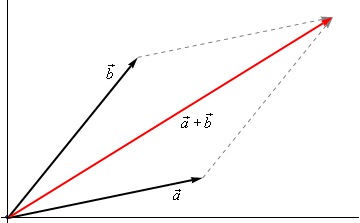
This is sometimes called the parallelogram law or triangle law.
Computationally, subtraction is very similar. Given the vectors \(\vec a = \left\langle {{a_1},{a_2},{a_3}} \right\rangle \) and \(\vec b = \left\langle {{b_1},{b_2},{b_3}} \right\rangle \) the difference of the two vectors is given by,
Here is the geometric interpretation of the difference of two vectors.
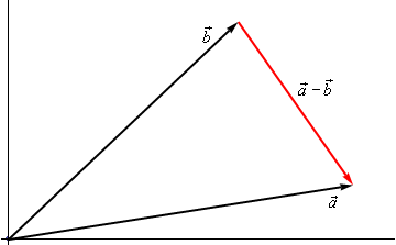
It is a little harder to see this geometric interpretation. To help see this let’s instead think of subtraction as the addition of \(\vec a\) and \( - \,\vec b\). First, as we’ll see in a bit \( - \,\vec b\) is the same vector as \(\vec b\) with opposite signs on all the components. In other words, \( - \,\vec b\) goes in the opposite direction as \(\vec b\). Here is the vector set up for \(\vec a + \left( { - \vec b} \right)\).
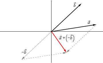
As we can see from this figure we can move the vector representing \(\vec a + \left( { - \vec b} \right)\) to the position we’ve got in the first figure showing the difference of the two vectors.
Note that we can’t add or subtract two vectors unless they have the same number of components. If they don’t have the same number of components then addition and subtraction can’t be done.
The next arithmetic operation that we want to look at is scalar multiplication. Given the vector \(\vec a = \left\langle {{a_1},{a_2},{a_3}} \right\rangle \) and any number \(c\) the scalar multiplication is,
So, we multiply all the components by the constant \(c\). To see the geometric interpretation of scalar multiplication let’s take a look at an example.
Here are the three scalar multiplications.
\[3\vec a = \left\langle {6,12} \right\rangle \hspace{0.25in}\hspace{0.25in}\frac{1}{2}\vec a = \left\langle {1,2} \right\rangle \hspace{0.25in}\hspace{0.25in} - 2\vec a = \left\langle { - 4, - 8} \right\rangle \]Here is the graph for each of these vectors.
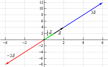
In the previous example we can see that if \(c\) is positive all scalar multiplication will do is stretch (if \(c > 1\)) or shrink (if \(c < 1\)) the original vector, but it won’t change the direction. Likewise, if \(c\) is negative scalar multiplication will switch the direction so that the vector will point in exactly the opposite direction and it will again stretch or shrink the magnitude of the vector depending upon the size of \(c\).
There are several nice applications of scalar multiplication that we should now take a look at.
The first is parallel vectors. This is a concept that we will see quite a bit over the next couple of sections. Two vectors are parallel if they have the same direction or are in exactly opposite directions. Now, recall again the geometric interpretation of scalar multiplication. When we performed scalar multiplication we generated new vectors that were parallel to the original vectors (and each other for that matter).
So, let’s suppose that \(\vec a\) and \(\vec b\) are parallel vectors. If they are parallel then there must be a number \(c\) so that,
\[\vec a = c\vec b\]So, two vectors are parallel if one is a scalar multiple of the other.
- \(\vec a = \left\langle {2, - 4,1} \right\rangle ,\,\,\vec b = \left\langle { - 6,12, - 3} \right\rangle \)
- \(\vec a = \left\langle {4,10} \right\rangle ,\,\,\vec b = \left\langle {2, - 9} \right\rangle \)
These two vectors are parallel since \(\vec b = - 3\vec a\)
b \(\vec a = \left\langle {4,10} \right\rangle ,\,\,\vec b = \left\langle {2, - 9} \right\rangle \) Show Solution
These two vectors aren’t parallel. This can be seen by noticing that \(4\left( {\frac{1}{2}} \right) = 2\) and yet \(10\left( {\frac{1}{2}} \right) = 5 \ne - 9\). In other words, we can’t make \(\vec a\) be a scalar multiple of \(\vec b\).
The next application is best seen in an example.
Okay, what we’re asking for is a new parallel vector (points in the same direction) that happens to be a unit vector. We can do this with a scalar multiplication since all scalar multiplication does is change the length of the original vector (along with possibly flipping the direction to the opposite direction).
Here’s what we’ll do. First let’s determine the magnitude of \(\vec w\).
\[\left\| {\vec w} \right\| = \sqrt {25 + 4 + 1} = \sqrt {30} \]Now, let’s form the following new vector,
\[\vec u = \frac{1}{{\left\| {\vec w} \right\|}}\vec w = \frac{1}{{\sqrt {30} }}\left\langle { - 5,2,1} \right\rangle = \left\langle { - \frac{5}{{\sqrt {30} }},\frac{2}{{\sqrt {30} }},\frac{1}{{\sqrt {30} }}} \right\rangle \]The claim is that this is a unit vector. That’s easy enough to check
\[\left\| {\vec u} \right\| = \sqrt {\frac{{25}}{{30}} + \frac{4}{{30}} + \frac{1}{{30}}} = \sqrt {\frac{{30}}{{30}}} = 1\]This vector also points in the same direction as \(\vec w\) since it is only a scalar multiple of \(\vec w\) and we used a positive multiple.
So, in general, given a vector \(\vec w\), \(\vec u = \frac{{\vec w}}{{\left\| {\vec w} \right\|}}\) will be a unit vector that points in the same direction as \(\vec w\).
Standard Basis Vectors Revisited
In the previous section we introduced the idea of standard basis vectors without really discussing why they were important. We can now do that. Let’s start with the vector
\[\vec a = \left\langle {{a_1},{a_2},{a_3}} \right\rangle \]We can use the addition of vectors to break this up as follows,
\[\begin{align*}\vec a & = \left\langle {{a_1},{a_2},{a_3}} \right\rangle \\ & = \left\langle {{a_1},0,0} \right\rangle + \left\langle {0,{a_2},0} \right\rangle + \left\langle {0,0,{a_3}} \right\rangle \end{align*}\]Using scalar multiplication we can further rewrite the vector as,
\[\begin{align*}\vec a & = \left\langle {{a_1},0,0} \right\rangle + \left\langle {0,{a_2},0} \right\rangle + \left\langle {0,0,{a_3}} \right\rangle \\ & = {a_1}\left\langle {1,0,0} \right\rangle + {a_2}\left\langle {0,1,0} \right\rangle + {a_3}\left\langle {0,0,1} \right\rangle \end{align*}\]Finally, notice that these three new vectors are simply the three standard basis vectors for three dimensional space.
\[\left\langle {{a_1},{a_2},{a_3}} \right\rangle = {a_1}\vec i + {a_2}\vec j + {a_3}\vec k\]So, we can take any vector and write it in terms of the standard basis vectors. From this point on we will use the two notations interchangeably so make sure that you can deal with both notations.
In order to do the problem we’ll convert to one notation and then perform the indicated operations.
\[\begin{align*}2\vec a - 3\vec w & = 2\left\langle {3, - 9,1} \right\rangle - 3\left\langle { - 1,0,8} \right\rangle \\ & = \left\langle {6, - 18,2} \right\rangle - \left\langle { - 3,0,24} \right\rangle \\ & = \left\langle {9, - 18, - 22} \right\rangle \end{align*}\]We will leave this section with some basic properties of vector arithmetic.
Properties
If \(\vec v\), \(\vec w\) and \(\vec u\) are vectors (each with the same number of components) and \(a\) and \(b\) are two numbers then we have the following properties.
\[\begin{array}{ll}\vec v + \vec w = \vec w + \vec v \hspace{0.75in} & \vec u + \left( {\vec v + \vec w} \right) = \left( {\vec u + \vec v} \right) + \vec w\\ \vec v + \vec 0 = \vec v \hspace{0.75in} & 1\vec v = \vec v\\ a\left( {\vec v + \vec w} \right) = a\vec v + a\vec w \hspace{0.75in} & \left( {a + b} \right)\vec v = a\vec v + b\vec v\end{array}\]The proofs of these are pretty much just “computation” proofs so we’ll prove one of them and leave the others to you to prove.
Proof of \(a\left( {\vec v + \vec w} \right) = a\vec v + a\vec w\)
We’ll start with the two vectors, \(\vec v = \left\langle {{v_1},{v_2}, \ldots ,{v_n}} \right\rangle \) and \(\vec w = \left\langle {{w_1},{w_2}, \ldots ,{w_n}} \right\rangle \) and yes we did mean for these to each have \(n\) components. The theorem works for general vectors so we may as well do the proof for general vectors.
Now, as noted above this is pretty much just a “computational” proof. What that means is that we’ll compute the left side and then do some basic arithmetic on the result to show that we can make the left side look like the right side. Here is the work.
\[\begin{align*}a\left( {\vec v + \vec w} \right) & = a\left( {\left\langle {{v_1},{v_2}, \ldots ,{v_n}} \right\rangle + \left\langle {{w_1},{w_2}, \ldots ,{w_n}} \right\rangle } \right)\\ & = a\left\langle {{v_1} + {w_1},{v_2} + {w_2}, \ldots ,{v_n} + {w_n}} \right\rangle \\ & = \left\langle {a\left( {{v_1} + {w_1}} \right),a\left( {{v_2} + {w_2}} \right), \ldots ,a\left( {{v_n} + {w_n}} \right)} \right\rangle \\ & = \left\langle {a{v_1} + a{w_1},a{v_2} + a{w_2}, \ldots ,a{v_n} + a{w_n}} \right\rangle \\ & = \left\langle {a{v_1},a{v_2}, \ldots ,a{v_n}} \right\rangle + \left\langle {a{w_1},a{w_2}, \ldots ,a{w_n}} \right\rangle \\ & = a\left\langle {{v_1},{v_2}, \ldots ,{v_n}} \right\rangle + a\left\langle {{w_1},{w_2}, \ldots ,{w_n}} \right\rangle = a\vec v + a\vec w\end{align*}\]