In this section we need to take a look at the equation of a line in .  As we saw in the previous section the equation  does not describe a line in , instead it describes a plane. This doesn’t mean however that we can’t write down an equation for a line in 3-D space.  We’re just going to need  a new way of writing down the equation of a curve.

So, before we get into the equations of lines we first need to briefly look at vector functions.  We’re going to take a more in depth look at vector functions later.  At this point all that we need to worry about is notational issues and how they can be used to give the equation of a curve.

The best way to get an idea of what a vector function is and what its graph looks like is to look at an example.  So, consider the following vector function.

A vector function is a function that takes one or more variables, one in this case, and returns a vector.  Note as well that a vector function can be a function of two or more variables.  However, in those cases the graph may no longer be a curve in space.

The vector that the function gives can be a vector in whatever dimension we need it to be.  In the example above it returns a vector in .  When we get to the real subject of this section, equations of lines, we’ll be using a vector function that returns a vector in  

Now, we want to determine the graph of the vector function above.  In order to find the graph of our function we’ll think of the vector that the vector function returns as a position vector for points on the graph.  Recall that a position vector, say , is a vector that starts at the origin and ends at the point . 

So, to get the graph of a vector function all we need to do is plug in some values of the variable and then plot the point that corresponds to each position vector we get out of the function and play connect the dots.  Here are some evaluations for our example.

So, each of these are position vectors representing points on the graph of our vector function.  The points,

 are all points that lie on the graph of our vector function.

If we do some more evaluations and plot all the points we get the following sketch.

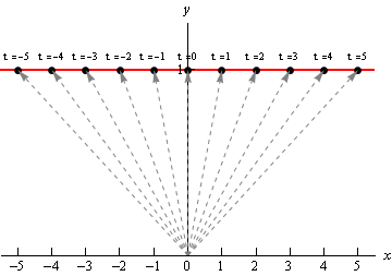
In this sketch we’ve included the position vector (in gray and dashed) for several evaluations as well as the t (above each point) we used for each evaluation.  It looks like, in this case the graph of the vector equation is in fact the line .

Here’s another quick example.  Here is the graph of .

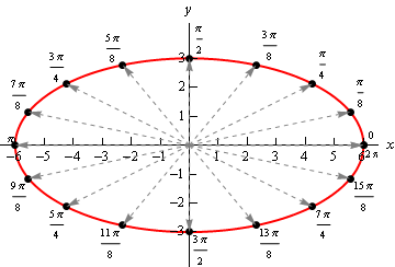
In this case we get an ellipse.  It is important to not come away from this section with the idea that vector functions only graph out lines.  We’ll be looking at lines in this section, but the graphs of vector functions do not have to be lines as the example above shows.

We’ll leave this brief discussion of vector functions with another way to think of the graph of a vector function.   Imagine that a pencil/pen is attached to the end of the position vector and as we increase the variable the resulting position vector moves and as it moves the pencil/pen on the end sketches out the curve for the vector function.

Okay, we now need to move into the actual topic of this section.  We want to write down the equation of a line in  and as suggested by the work above we will need a vector function to do this.  To see how we’re going to do this let’s think about what we need to write down the equation of a line in .  In two dimensions we need the slope (m) and a point that was on the line in order to write down the equation.

In  that is still all that we need except in this case the “slope” won’t be a simple number as it was in two dimensions.  In this case we will need to acknowledge that a line can have a three dimensional slope.  So, we need something that will allow us to describe a direction that is potentially in three dimensions.  We already have a quantity that will do this for us.  Vectors give directions and can be three dimensional objects. 

So, let’s start with the following information.  Suppose that we know a point that is on the line, , and that  is some vector that is parallel to the line.  Note, in all likelihood,  will not be on the line itself.  We only need  to be parallel to the line.  Finally, let  be any point on the line.

Now, since our “slope” is a vector let’s also represent the two points on the line as vectors.  We’ll do this with position vectors.  So, let  and  be the position vectors for P₀ and P respectively.  Also, for no apparent reason, let’s define  to be the vector with representation .

We now have the following sketch with all these points and vectors on it.

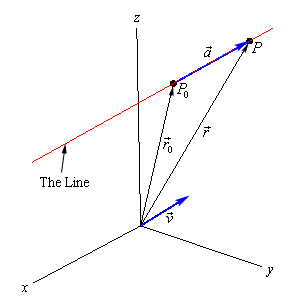
Now, we’ve shown the parallel vector, , as a position vector but it doesn’t need to be a position vector.  It can be anywhere, a position vector, on the line or off the line, it just needs to be parallel to the line.

Next, notice that we can write  as follows,

If you’re not sure about this go back and check out the sketch for vector addition in the vector arithmetic section.  Now, notice that the vectors  and  are parallel.  Therefore there is a number, t, such that

We now have,

This is called the vector form of the equation of a line.  The only part of this equation that is not known is the t.  Notice that  will be a vector that lies along the line and it tells us how far from the original point that we should move.  If t is positive we move away from the original point in the direction of  (right in our sketch)  and if t is negative we move away from the original point in the opposite direction of  (left in our sketch).  As t varies over all possible values we will completely cover the line.  The following sketch shows this dependence on t of our sketch.

There are several other forms of the equation of a line.  To get the first alternate form let’s start with the vector form and do a slight rewrite.

The only way for two vectors to be equal is for the components to be equal. In other words,

This set of equations is called the parametric form of the equation of a line.  Notice as well that this is really nothing more than an extension of the parametric equations we’ve seen previously.  The only difference is that we are now working in three dimensions instead of two dimensions.

To get a point on the line all we do is pick a t and plug into either form of the line.  In the vector form of the line we get a position vector for the point and in the parametric form we get the actual coordinates of the point.

There is one more form of the line that we want to look at.  If we assume that a, b, and c are all non-zero numbers we can solve each of the equations in the parametric form of the line for t.  We can then set all of them equal to each other since t will be the same number in each.  Doing this gives the following,

This is called the symmetric equations of the line. 

If one of a, b, or c does happen to be zero we can still write down the symmetric equations.  To see this let’s suppose that .  In this case t will not exist in the parametric equation for y and so we will only solve the parametric equations for x and z for t.  We then set those equal and acknowledge the parametric equation for y as follows,

Let’s take a look at an example.