Section 7.10 : Approximating Definite Integrals
In this chapter we’ve spent quite a bit of time on computing the values of integrals. However, not all integrals can be computed. A perfect example is the following definite integral.
\[\int_{{\,0}}^{{\,2}}{{{{\bf{e}}^{{x^2}}}\,dx}}\]We now need to talk a little bit about estimating values of definite integrals. We will look at three different methods, although one should already be familiar to you from your Calculus I days. We will develop all three methods for estimating
\[\int_{{\,a}}^{{\,b}}{{f\left( x \right)\,dx}}\]by thinking of the integral as an area problem and using known shapes to estimate the area under the curve.
Let’s get first develop the methods and then we’ll try to estimate the integral shown above.
Midpoint Rule
This is the rule that should be somewhat familiar to you. We will divide the interval \(\left[ {a,b} \right]\) into \(n\) subintervals of equal width,
\[\Delta x = \frac{{b - a}}{n}\]We will denote each of the intervals as follows,
\[\left[ {{x_0},{x_1}} \right],\,\,\left[ {{x_1},{x_2}} \right], \ldots ,\left[ {{x_{n - 1}},{x_n}} \right]\hspace{0.25in}{\mbox{where}}\,{x_0} = a{\mbox{ and }}{x_n} = b\]Then for each interval let \(x_i^*\) be the midpoint of the interval. We then sketch in rectangles for each subinterval with a height of \(f\left( {x_i^*} \right)\). Here is a graph showing the set up using \(n = 6\).
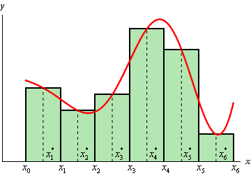
We can easily find the area for each of these rectangles and so for a general \(n\) we get that,
\[\int_{{\,a}}^{{\,b}}{{f\left( x \right)\,dx}} \approx \Delta x\,f\left( {x_1^*} \right) + \Delta x\,f\left( {x_2^*} \right) + \cdots + \Delta x\,f\left( {x_n^*} \right)\]Or, upon factoring out a \(\Delta x\) we get the general Midpoint Rule.
\[\int_{{\,a}}^{{\,b}}{{f\left( x \right)\,dx}} \approx \Delta x\left[f\left( {x_1^*} \right) + f\left( {x_2^*} \right) + \cdots + f\left( {x_n^*} \right)\right]\]Trapezoid Rule
For this rule we will do the same set up as for the Midpoint Rule. We will break up the interval \(\left[ {a,b} \right]\) into \(n\) subintervals of width,
\[\Delta x = \frac{{b - a}}{n}\]Then on each subinterval we will approximate the function with a straight line that is equal to the function values at either endpoint of the interval. Here is a sketch of this case for \(n = 6\).
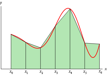
Each of these objects is a trapezoid (hence the rule’s name…) and as we can see some of them do a very good job of approximating the actual area under the curve and others don’t do such a good job.
The area of the trapezoid in the interval \(\left[ {{x_{i - 1}},{x_i}} \right]\) is given by,
\[{A_{\,i}} = \frac{{\Delta x}}{2}\left( {f\left( {{x_{i - 1}}} \right) + f\left( {{x_i}} \right)} \right)\]So, if we use \(n\) subintervals the integral is approximately,
\[\int_{{\,a}}^{{\,b}}{{f\left( x \right)\,dx}} \approx \frac{{\Delta x}}{2}\left( {f\left( {{x_0}} \right) + f\left( {{x_1}} \right)} \right) + \frac{{\Delta x}}{2}\left( {f\left( {{x_1}} \right) + f\left( {{x_2}} \right)} \right) + \cdots + \frac{{\Delta x}}{2}\left( {f\left( {{x_{n - 1}}} \right) + f\left( {{x_n}} \right)} \right)\]Upon doing a little simplification we arrive at the general Trapezoid Rule.
\[\int_{{\,a}}^{{\,b}}{{f\left( x \right)\,dx}} \approx \frac{{\Delta x}}{2} \left[ f\left( {{x_0}} \right) + 2f\left( {{x_1}} \right) + 2f\left( {{x_2}} \right) + \cdots + 2f\left( {{x_{n - 1}}} \right) + f\left( {{x_n}} \right) \right]\]Note that all the function evaluations, with the exception of the first and last, are multiplied by 2.
Simpson’s Rule
This is the final method we’re going to take a look at and in this case we will again divide up the interval \(\left[ {a,b} \right]\) into \(n\) subintervals. However, unlike the previous two methods we need to require that \(n\) be even. The reason for this will be evident in a bit. The width of each subinterval is,
\[\Delta x = \frac{{b - a}}{n}\]In the Trapezoid Rule we approximated the curve with a straight line. For Simpson’s Rule we are going to approximate the function with a quadratic and we’re going to require that the quadratic agree with three of the points from our subintervals. Below is a sketch of this using \(n = 6\). Each of the approximations is colored differently so we can see how they actually work.
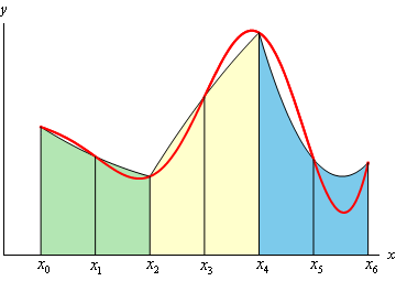
Notice that each approximation actually covers two of the subintervals. This is the reason for requiring \(n\) to be even. Some of the approximations look more like a line than a quadratic, but they really are quadratics. Also note that some of the approximations do a better job than others. It can be shown that the area under the approximation on the intervals \(\left[ {{x_{i - 1}},{x_i}} \right]\) and \(\left[ {{x_i},{x_{i + 1}}} \right]\) is,
\[{A_{\,i}} = \frac{{\Delta x}}{3}\left( {f\left( {{x_{i - 1}}} \right) + 4f\left( {{x_i}} \right) + f\left( {{x_{i + 1}}} \right)} \right)\]If we use \(n\) subintervals the integral is then approximately,
\[\begin{align*}\int_{{\,a}}^{{\,b}}{{f\left( x \right)\,dx}} & \approx \frac{{\Delta x}}{3}\left( {f\left( {{x_0}} \right) + 4f\left( {{x_1}} \right) + f\left( {{x_2}} \right)} \right) + \frac{{\Delta x}}{3}\left( {f\left( {{x_2}} \right) + 4f\left( {{x_3}} \right) + f\left( {{x_4}} \right)} \right)\\ & \hspace{1.5in} + \cdots + \frac{{\Delta x}}{3}\left( {f\left( {{x_{n - 2}}} \right) + 4f\left( {{x_{n - 1}}} \right) + f\left( {{x_n}} \right)} \right)\end{align*}\]Upon simplifying we arrive at the general Simpson’s Rule.
\[\int_{{\,a}}^{{\,b}}{{f\left( x \right)\,dx}} \approx \frac{{\Delta x}}{3} \left[ f\left( {{x_0}} \right) + 4f\left( {{x_1}} \right) + 2f\left( {{x_2}} \right) + \cdots + 2f\left( {{x_{n - 2}}} \right) + 4f\left( {{x_{n - 1}}} \right) + f\left( {{x_n}} \right) \right]\]In this case notice that all the function evaluations at points with odd subscripts are multiplied by 4 and all the function evaluations at points with even subscripts (except for the first and last) are multiplied by 2. If you can remember this, this is a fairly easy rule to remember.
Okay, it’s time to work an example and see how these rules work.
First, for reference purposes, Mathematica gives the following value for this integral.
\[\int_{{\,0}}^{{\,2}}{{{{\bf{e}}^{{x^2}}}\,dx}} = 16.45262776\]In each case the width of the subintervals will be,
\[\Delta x = \frac{{2 - 0}}{4} = \frac{1}{2}\]and so the subintervals will be,
\[\left[ {0,\,\,0.5} \right],\,\,\left[ {0.5,\,\,1} \right],\,\,\left[ {1,\,\,1.5} \right],\,\,\left[ {1.5,\,\,2} \right]\]Let’s go through each of the methods.
Midpoint Rule
\[\int_{{\,0}}^{{\,2}}{{{{\bf{e}}^{{x^2}}}\,dx}} \approx \frac{1}{2}\left( {{{\bf{e}}^{{{\left( {0.25} \right)}^2}}} + {{\bf{e}}^{{{\left( {0.75} \right)}^2}}} + {{\bf{e}}^{{{\left( {1.25} \right)}^2}}} + {{\bf{e}}^{{{\left( {1.75} \right)}^2}}}} \right) = 14.48561253\]Remember that we evaluate at the midpoints of each of the subintervals here! The Midpoint Rule has an error of 1.96701523.
Trapezoid Rule
\[\int_{{\,0}}^{{\,2}}{{{{\bf{e}}^{{x^2}}}\,dx}} \approx \frac{{{1}/{2}\;}}{2}\left( {{{\bf{e}}^{{{\left( 0 \right)}^2}}} + 2{{\bf{e}}^{{{\left( {0.5} \right)}^2}}} + 2{{\bf{e}}^{{{\left( 1 \right)}^2}}} + 2{{\bf{e}}^{{{\left( {1.5} \right)}^2}}} + {{\bf{e}}^{{{\left( 2 \right)}^2}}}} \right) = 20.64455905\]The Trapezoid Rule has an error of 4.19193129
Simpson’s Rule
\[\int_{{\,0}}^{{\,2}}{{{{\bf{e}}^{{x^2}}}\,dx}} \approx \frac{{{1}/{2}\;}}{3}\left( {{{\bf{e}}^{{{\left( 0 \right)}^2}}} + 4{{\bf{e}}^{{{\left( {0.5} \right)}^2}}} + 2{{\bf{e}}^{{{\left( 1 \right)}^2}}} + 4{{\bf{e}}^{{{\left( {1.5} \right)}^2}}} + {{\bf{e}}^{{{\left( 2 \right)}^2}}}} \right) = 17.35362645\]The Simpson’s Rule has an error of 0.90099869.
None of the estimations in the previous example are all that good. The best approximation in this case is from the Simpson’s Rule and yet it still had an error of almost 1. To get a better estimation we would need to use a larger \(n\). So, for completeness sake here are the estimates for some larger value of \(n\).
| Midpoint | Trapezoid | Simpson’s | ||||
| \(n\) | Approx. | Error | Approx. | Error | Approx. | Error |
| 8 | 15.9056767 | 0.5469511 | 17.5650858 | 1.1124580 | 16.5385947 | 0.0859669 |
| 16 | 16.3118539 | 0.1407739 | 16.7353812 | 0.2827535 | 16.4588131 | 0.0061853 |
| 32 | 16.4171709 | 0.0354568 | 16.5236176 | 0.0709898 | 16.4530297 | 0.0004019 |
| 64 | 16.4437469 | 0.0088809 | 16.4703942 | 0.0177665 | 16.4526531 | 0.0000254 |
| 128 | 16.4504065 | 0.0022212 | 16.4570706 | 0.0044428 | 16.4526294 | 0.0000016 |
In this case we were able to determine the error for each estimate because we could get our hands on the exact value. Often this won’t be the case and so we’d next like to look at error bounds for each estimate.
These bounds will give the largest possible error in the estimate, but it should also be pointed out that the actual error may be significantly smaller than the bound. The bound is only there so we can say that we know the actual error will be less than the bound.
So, suppose that \(\left| {f''\left( x \right)} \right| \le K\) and \(\left| {{f^{\left( 4 \right)}}\left( x \right)} \right| \le M\) for \(a \le x \le b\) then if \({E_M}\), \({E_T}\), and \({E_S}\) are the actual errors for the Midpoint, Trapezoid and Simpson’s Rule we have the following bounds,
\[\left| {{E_M}} \right| \le \frac{{K{{\left( {b - a} \right)}^3}}}{{24{n^2}}}\hspace{0.25in}\left| {{E_T}} \right| \le \frac{{K{{\left( {b - a} \right)}^3}}}{{12{n^2}}}\hspace{0.25in}\left| {{E_S}} \right| \le \frac{{M{{\left( {b - a} \right)}^5}}}{{180{n^4}}}\]We already know that \(n = 4\), \(a = 0\), and \(b = 2\) so we just need to compute \(K\) (the largest value of the second derivative) and \(M\) (the largest value of the fourth derivative). This means that we’ll need the second and fourth derivative of \(f\left( x \right)\).
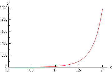
\[\begin{align*}f''\left( x \right) & = 2{{\bf{e}}^{{x^2}}}\left( {1 + 2{x^2}} \right)\\ {f^{\left( 4 \right)}}\left( x \right) & = 4{{\bf{e}}^{{x^2}}}\left( {3 + 12{x^2} + 4{x^4}} \right)\end{align*}\]Here is a graph of the second derivative.
Here is a graph of the fourth derivative.
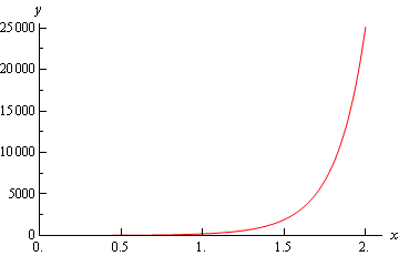
So, from these graphs it’s clear that the largest value of both of these are at \(x = 2\). So,
\[\begin{align*}f''\left( 2 \right) & = 982.7667\hspace{0.25in}\hspace{0.25in} \Rightarrow \hspace{0.25in}\hspace{0.25in}K = 983\\ {f^{\left( 4 \right)}}\left( 2 \right) & = 25115.14901\hspace{0.25in} \Rightarrow \hspace{0.25in}\hspace{0.25in}M = 25116\end{align*}\]We rounded to make the computations simpler. Note however, that this does not need to be done.
Here are the bounds for each rule.
\[\left| {{E_M}} \right| \le \frac{{983{{\left( {2 - 0} \right)}^3}}}{{24{{\left( 4 \right)}^2}}} = 20.4791666667\] \[\left| {{E_T}} \right| \le \frac{{983{{\left( {2 - 0} \right)}^3}}}{{12{{\left( 4 \right)}^2}}} = 40.9583333333\] \[\left| {{E_S}} \right| \le \frac{{25116{{\left( {2 - 0} \right)}^5}}}{{180{{\left( 4 \right)}^4}}} = 17.4416666667\]In each case we can see that the errors are significantly smaller than the actual bounds.