Section 8.5 : Fourier Cosine Series
In this section we’re going to take a look at Fourier cosine series. We’ll start off much as we did in the previous section where we looked at Fourier sine series. Let’s start by assuming that the function, \(f\left( x \right)\), we’ll be working with initially is an even function (i.e. \(f\left( { - x} \right) = f\left( x \right)\)) and that we want to write a series representation for this function on \( - L \le x \le L\) in terms of cosines (which are also even). In other words, we are going to look for the following,
\[f\left( x \right) = \sum\limits_{n = 0}^\infty {{A_n}\cos \left( {\frac{{n\,\pi x}}{L}} \right)} \]This series is called a Fourier cosine series and note that in this case (unlike with Fourier sine series) we’re able to start the series representation at \(n = 0\) since that term will not be zero as it was with sines. Also, as with Fourier Sine series, the argument of \(\frac{{n\pi x}}{L}\) in the cosines is being used only because it is the argument that we’ll be running into in the next chapter. The only real requirement here is that the given set of functions we’re using be orthogonal on the interval we’re working on.
Note as well that we’re assuming that the series will in fact converge to \(f\left( x \right)\) on \( - L \le x \le L\) at this point. In a later section we’ll be looking into the convergence of this series in more detail.
So, to determine a formula for the coefficients, \({A_n}\), we’ll use the fact that \(\left\{ {\cos \left( {\frac{{n\pi x}}{L}} \right)} \right\}_{n\,\, = \,\,0}^\infty \) do form an orthogonal set on the interval \( - L \le x \le L\) as we showed in a previous section. In that section we also derived the following formula that we’ll need in a bit.
\[\int_{{ - L}}^{L}{{\cos \left( {\frac{{n\pi x}}{L}} \right)\cos \left( {\frac{{m\pi x}}{L}} \right)\,dx}} = \left\{ {\begin{array}{*{20}{l}}{2L}&{{\mbox{if }}n = m = 0}\\L&{{\mbox{if }}n = m \ne 0}\\0&{{\mbox{if }}n \ne m}\end{array}} \right.\]We’ll get a formula for the coefficients in almost exactly the same fashion that we did in the previous section. We’ll start with the representation above and multiply both sides by \(\cos \left( {\frac{{m\pi x}}{L}} \right)\) where \(m\) is a fixed integer in the range \(\left\{ {0,1,2,3, \ldots } \right\}\). Doing this gives,
\[f\left( x \right)\cos \left( {\frac{{m\,\pi x}}{L}} \right) = \sum\limits_{n = 0}^\infty {{A_n}\cos \left( {\frac{{n\,\pi x}}{L}} \right)\cos \left( {\frac{{m\,\pi x}}{L}} \right)} \]Next, we integrate both sides from \(x = - L\) to \(x = L\) and as we were able to do with the Fourier Sine series we can again interchange the integral and the series.
\[\begin{align*}\int_{{\, - L}}^{{\,L}}{{f\left( x \right)\cos \left( {\frac{{m\,\pi x}}{L}} \right)\,dx}} & = \int_{{\, - L}}^{L}{{\sum\limits_{n = 0}^\infty {{A_n}\cos \left( {\frac{{n\,\pi x}}{L}} \right)\cos \left( {\frac{{m\,\pi x}}{L}} \right)} }}\,dx\\ & = \sum\limits_{n = 0}^\infty {{A_n}\int_{{\, - L}}^{{\,L}}{{\cos \left( {\frac{{n\,\pi x}}{L}} \right)\cos \left( {\frac{{m\,\pi x}}{L}} \right)\,dx}}} \end{align*}\]We now know that the all of the integrals on the right side will be zero except when \(n = m\) because the set of cosines form an orthogonal set on the interval \( - L \le x \le L\). However, we need to be careful about the value of \(m\) (or \(n\) depending on the letter you want to use). So, after evaluating all of the integrals we arrive at the following set of formulas for the coefficients.
\(m = 0\):\[\int_{{\, - L}}^{{\,L}}{{f\left( x \right)dx}} = {A_{\,0}}\left( {2L} \right)\hspace{0.25in}\,\,\,\,\,\,\,\, \Rightarrow \hspace{0.25in}\,\,\,\,\,\,\,\,{A_{\,0}} = \frac{1}{{2L}}\int_{{\, - L}}^{{\,L}}{{f\left( x \right)\,dx}}\] \(m \ne 0\):
\[\int_{{\, - L}}^{{\,L}}{{f\left( x \right)\cos \left( {\frac{{m\,\pi x}}{L}} \right)\,dx}} = {A_{\,m}}\left( L \right)\hspace{0.25in}\,\,\,\,\,\,\,\, \Rightarrow \hspace{0.25in}\,\,\,\,\,\,\,\,{A_{\,m}} = \frac{1}{L}\int_{{\, - L}}^{{\,L}}{{f\left( x \right)\cos \left( {\frac{{m\,\pi x}}{L}} \right)\,dx}}\]
Summarizing everything up then, the Fourier cosine series of an even function, \(f\left( x \right)\) on \( - L \le x \le L\) is given by,
\[f\left( x \right)=\sum\limits_{n=0}^{\infty }{{{A}_{n}}\cos \left( \frac{n\,\pi x}{L} \right)} \hspace{0.25in} {{A}_{n}}=\left\{ \begin{array}{*{35}{l}} \displaystyle \frac{1}{2L}\int_{\,-L}^{\,L}{f\left( x \right)\,dx} & \,\,\,\,\,n=0 \\ \displaystyle \frac{1}{L}\int_{\,-L}^{\,L}{f\left( x \right)\cos \left( \frac{n\,\pi x}{L} \right)\,dx} & \,\,\,\,\,n\ne 0 \\ \end{array} \right.\]Finally, before we work an example, let’s notice that because both \(f\left( x \right)\) and the cosines are even the integrand in both of the integrals above is even and so we can write the formulas for the \({A_n}\)’s as follows,
\[{A_n} = \left\{ {\begin{array}{*{20}{l}}{\displaystyle \frac{1}{L}\int_{{\,0}}^{{\,L}}{{f\left( x \right)\,dx}}}&{\,\,\,\,\,n = 0}\\{\displaystyle \frac{2}{L}\int_{{\,0}}^{{\,L}}{{f\left( x \right)\cos \left( {\frac{{n\,\pi x}}{L}} \right)\,dx}}}&{\,\,\,\,\,n \ne 0}\end{array}} \right.\]Now let’s take a look at an example.
We clearly have an even function here and so all we really need to do is compute the coefficients and they are liable to be a little messy because we’ll need to do integration by parts twice. We’ll leave most of the actual integration details to you to verify.
\[{A_0} = \frac{1}{L}\int_{{\,0}}^{{\,L}}{{f\left( x \right)\,dx}} = \frac{1}{L}\int_{{\,0}}^{{\,L}}{{{x^2}\,dx}} = \frac{1}{L}\left( {\frac{{{L^3}}}{3}} \right) = \frac{{{L^2}}}{3}\] \[\begin{align*}{A_n} & = \frac{2}{L}\int_{{\,0}}^{{\,L}}{{f\left( x \right)\cos \left( {\frac{{n\,\pi x}}{L}} \right)\,dx}} = \frac{2}{L}\int_{{\,0}}^{{\,L}}{{{x^2}\cos \left( {\frac{{n\,\pi x}}{L}} \right)\,dx}}\\ & = \frac{2}{L}\left. {\left( {\frac{L}{{{n^3}{\pi ^3}}}} \right)\left( {2Ln\pi x\cos \left( {\frac{{n\,\pi x}}{L}} \right) + \left( {{n^2}{\pi ^2}{x^2} - 2{L^2}} \right)\sin \left( {\frac{{n\,\pi x}}{L}} \right)} \right)} \right|_0^L\\ & = \frac{2}{{{n^3}{\pi ^3}}}\left( {2{L^2}n\pi \cos \left( {n\,\pi } \right) + \left( {{n^2}{\pi ^2}{L^2} - 2{L^2}} \right)\sin \left( {n\,\pi } \right)} \right)\\ & = \frac{{4{L^2}{{\left( { - 1} \right)}^n}}}{{{n^2}{\pi ^2}}}\hspace{0.25in}\hspace{0.25in}n = 1,2,3, \ldots \end{align*}\]The coefficients are then,
\[{A_0} = \frac{{{L^2}}}{3}\hspace{0.25in}{A_n} = \frac{{4{L^2}{{\left( { - 1} \right)}^n}}}{{{n^2}{\pi ^2}}},\,\,\,\,n = 1,2,3, \ldots \]The Fourier cosine series is then,
\[{x^2} = \sum\limits_{n = 0}^\infty {{A_n}\cos \left( {\frac{{n\,\pi x}}{L}} \right)} = {A_0} + \sum\limits_{n = 1}^\infty {{A_n}\cos \left( {\frac{{n\,\pi x}}{L}} \right)} = \frac{{{L^2}}}{3} + \sum\limits_{n = 1}^\infty {\frac{{4{L^2}{{\left( { - 1} \right)}^n}}}{{{n^2}{\pi ^2}}}\cos \left( {\frac{{n\,\pi x}}{L}} \right)} \]Note that we’ll often strip out the \(n = 0\) from the series as we’ve done here because it will almost always be different from the other coefficients and it allows us to actually plug the coefficients into the series.
Now, just as we did in the previous section let’s ask what we need to do in order to find the Fourier cosine series of a function that is not even. As with Fourier sine series when we make this change we’ll need to move onto the interval \(0 \le x \le L\) now instead of \( - L \le x \le L\) and again we’ll assume that the series will converge to \(f\left( x \right)\) at this point and leave the discussion of the convergence of this series to a later section.
We could go through the work to find the coefficients here twice as we did with Fourier sine series, however there’s no real reason to. So, while we could redo all the work above to get formulas for the coefficients let’s instead go straight to the second method of finding the coefficients.
In this case, before we actually proceed with this we’ll need to define the even extension of a function, \(f\left( x \right)\) on \( - L \le x \le L\). So, given a function \(f\left( x \right)\) we’ll define the even extension of the function as,
\[g\left( x \right) = \left\{ {\begin{array}{*{20}{l}}{f\left( x \right)}&{\,\,\,\,{\mbox{if }}0 \le x \le L}\\{f\left( { - x} \right)}&{\,\,\,\,{\mbox{if }} - L \le x \le 0}\end{array}} \right.\]Showing that this is an even function is simple enough.
\[g\left( -x \right)=f\left( -\left( -x \right) \right)=f\left( x \right)=g\left( x \right) \hspace{0.25in} \text{for }0<x<L\]and we can see that \(g\left( x \right) = f\left( x \right)\) on \(0 \le x \le L\) and if \(f\left( x \right)\) is already an even function we get \(g\left( x \right) = f\left( x \right)\) on \( - L \le x \le L\).
Let’s take a look at some functions and sketch the even extensions for the functions.
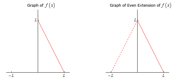
- \(f\left( x \right) = L - x\) on \(0 \le x \le L\)
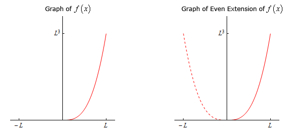
- \(f\left( x \right) = {x^3}\) on \(0 \le x \le L\)
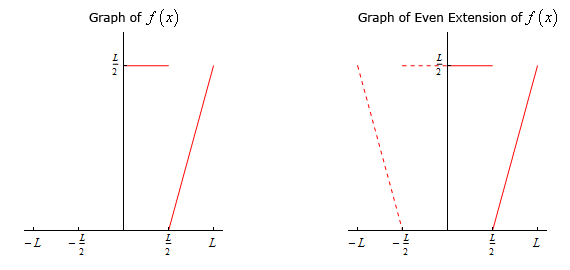
- \(f\left( x \right) = \left\{ {\begin{array}{*{20}{l}}{\frac{L}{2}}&{\,\,\,\,{\mbox{if }}0 \le x \le \frac{L}{2}}\\{x - \frac{L}{2}}&{\,\,\,\,{\mbox{if }}\frac{L}{2} \le x \le L}\end{array}} \right.\)
Here is the even extension of this function.
\[\begin{align*}g\left( x \right) & = \left\{ {\begin{array}{*{20}{l}}{f\left( x \right)}&{\,\,\,\,{\mbox{if }}0 \le x \le L}\\{f\left( { - x} \right)}&{\,\,\,\,{\mbox{if }} - L \le x \le 0}\end{array}} \right.\\ & = \left\{ {\begin{array}{*{20}{l}}{L - x}&{\,\,\,\,{\mbox{if }}0 \le x \le L}\\{L + x}&{\,\,\,\,{\mbox{if }} - L \le x \le 0}\end{array}} \right.\end{align*}\]Here is the graph of both the original function and its even extension. Note that we’ve put the “extension” in with a dashed line to make it clear the portion of the function that is being added to allow us to get the even extension
b \(f\left( x \right) = {x^3}\) on \(0 \le x \le L\) Show Solution
The even extension of this function is,
\[\begin{align*}g\left( x \right) & = \left\{ {\begin{array}{*{20}{l}}{f\left( x \right)}&{\,\,\,\,{\mbox{if }}0 \le x \le L}\\{f\left( { - x} \right)}&{\,\,\,\,{\mbox{if }} - L \le x \le 0}\end{array}} \right.\\ & = \left\{ {\begin{array}{*{20}{l}}{{x^3}}&{\,\,\,\,{\mbox{if }}0 \le x \le L}\\{ - {x^3}}&{\,\,\,\,{\mbox{if }} - L \le x \le 0}\end{array}} \right.\end{align*}\]The sketch of the function and the even extension is,
c \(f\left( x \right) = \left\{ {\begin{array}{*{20}{l}}{\frac{L}{2}}&{\,\,\,\,{\mbox{if }}0 \le x \le \frac{L}{2}}\\{x - \frac{L}{2}}&{\,\,\,\,{\mbox{if }}\frac{L}{2} \le x \le L}\end{array}} \right.\) Show Solution
Here is the even extension of this function,
\[\begin{align*}g\left( x \right) & = \left\{ {\begin{array}{*{20}{l}}{f\left( x \right)}&{\,\,\,\,{\mbox{if }}0 \le x \le L}\\{f\left( { - x} \right)}&{\,\,\,\,{\mbox{if }} - L \le x \le 0}\end{array}} \right.\\ & = \left\{ {\begin{array}{*{20}{l}}{x - \frac{L}{2}}&{\,\,\,\,{\mbox{if }}\frac{L}{2} \le x \le L}\\{\frac{L}{2}}&{\,\,\,\,{\mbox{if }}0 \le x \le \frac{L}{2}}\\{\frac{L}{2}}&{\,\,\,\,{\mbox{if }} - \frac{L}{2} \le x \le 0}\\{ - x - \frac{L}{2}}&{\,\,\,\,{\mbox{if }} - L \le x \le - \frac{L}{2}}\end{array}} \right.\end{align*}\]The sketch of the function and the even extension is,
Okay, let’s now think about how we can use the even extension of a function to find the Fourier cosine series of any function \(f\left( x \right)\) on \(0 \le x \le L\).
So, given a function \(f\left( x \right)\) we’ll let \(g\left( x \right)\) be the even extension as defined above. Now, \(g\left( x \right)\) is an even function on \( - L \le x \le L\) and so we can write down its Fourier cosine series. This is,
\[g\left( x \right) = \sum\limits_{n = 0}^\infty {{A_n}\cos \left( {\frac{{n\,\pi x}}{L}} \right)} \hspace{0.25in}{A_n} = \left\{ {\begin{array}{*{20}{l}}{\displaystyle \frac{1}{L}\int_{{\,0}}^{{\,L}}{{f\left( x \right)\,dx}}}&{\,\,\,\,\,n = 0}\\{\displaystyle \frac{2}{L}\int_{{\,0}}^{{\,L}}{{f\left( x \right)\cos \left( {\frac{{n\,\pi x}}{L}} \right)\,dx}}}&{\,\,\,\,\,n \ne 0}\end{array}} \right.\]and note that we’ll use the second form of the integrals to compute the constants.
Now, because we know that on \(0 \le x \le L\) we have \(f\left( x \right) = g\left( x \right)\) and so the Fourier cosine series of \(f\left( x \right)\) on \(0 \le x \le L\) is also given by,
\[f\left( x \right) = \sum\limits_{n = 0}^\infty {{A_n}\cos \left( {\frac{{n\,\pi x}}{L}} \right)} \hspace{0.25in}{A_n} = \left\{ {\begin{array}{*{20}{l}}{\displaystyle \frac{1}{L}\int_{{\,0}}^{{\,L}}{{f\left( x \right)\,dx}}}&{\,\,\,\,\,n = 0}\\{\displaystyle \frac{2}{L}\int_{{\,0}}^{{\,L}}{{f\left( x \right)\cos \left( {\frac{{n\,\pi x}}{L}} \right)\,dx}}}&{\,\,\,\,\,n \ne 0}\end{array}} \right.\]Let’s take a look at a couple of examples.
All we need to do is compute the coefficients so here is the work for that,
\[{A_0} = \frac{1}{L}\int_{{\,0}}^{{\,L}}{{f\left( x \right)\,dx}} = \frac{1}{L}\int_{{\,0}}^{{\,L}}{{L - x\,dx}} = \frac{L}{2}\] \[\begin{align*}{A_n} & = \frac{2}{L}\int_{{\,0}}^{{\,L}}{{f\left( x \right)\cos \left( {\frac{{n\,\pi x}}{L}} \right)\,dx}} = \frac{2}{L}\int_{{\,0}}^{{\,L}}{{\left( {L - x} \right)\cos \left( {\frac{{n\,\pi x}}{L}} \right)\,dx}}\\ & = \frac{2}{L}\left. {\left( {\frac{L}{{{n^2}{\pi ^2}}}} \right)\left( {n\pi \left( {L - x} \right)\sin \left( {\frac{{n\,\pi x}}{L}} \right) - L\cos \left( {\frac{{n\,\pi x}}{L}} \right)} \right)} \right|_0^L\\ & = \frac{2}{L}\left( {\frac{L}{{{n^2}{\pi ^2}}}} \right)\left( { - L\cos \left( {n\,\pi } \right) + L} \right) = \frac{{2L}}{{{n^2}{\pi ^2}}}\left( {1 + {{\left( { - 1} \right)}^{n + 1}}} \right)\hspace{0.25in}\hspace{0.25in}n = 1,2,3, \ldots \end{align*}\]The Fourier cosine series is then,
\[f\left( x \right) = \frac{L}{2} + \sum\limits_{n = 1}^\infty {\frac{{2L}}{{{n^2}{\pi ^2}}}\left( {1 + {{\left( { - 1} \right)}^{n + 1}}} \right)\cos \left( {\frac{{n\,\pi x}}{L}} \right)} \]Note that as we did with the first example in this section we stripped out the \({A_0}\) term before we plugged in the coefficients.
Next, let’s find the Fourier cosine series of an odd function. Note that this is doable because we are really finding the Fourier cosine series of the even extension of the function.
The integral for \({A_0}\) is simple enough but the integral for the rest will be fairly messy as it will require three integration by parts. We’ll leave most of the details of the actual integration to you to verify. Here’s the work,
\[{A_0} = \frac{1}{L}\int_{{\,0}}^{{\,L}}{{f\left( x \right)\,dx}} = \frac{1}{L}\int_{{\,0}}^{{\,L}}{{{x^3}\,dx}} = \frac{{{L^3}}}{4}\] \[\begin{align*}{A_n} & = \frac{2}{L}\int_{{\,0}}^{{\,L}}{{f\left( x \right)\cos \left( {\frac{{n\,\pi x}}{L}} \right)\,dx}} = \frac{2}{L}\int_{{\,0}}^{{\,L}}{{{x^3}\cos \left( {\frac{{n\,\pi x}}{L}} \right)\,dx}}\\ & = \frac{2}{L}\left. {\left( {\frac{L}{{{n^4}{\pi ^4}}}} \right)\left( {n\pi x\left( {{n^2}{\pi ^2}{x^2} - 6{L^2}} \right)\sin \left( {\frac{{n\,\pi x}}{L}} \right) + \left( {3L{n^2}{\pi ^2}{x^2} - 6{L^3}} \right)\cos \left( {\frac{{n\,\pi x}}{L}} \right)} \right)} \right|_0^L\\ & = \frac{2}{L}\left( {\frac{L}{{{n^4}{\pi ^4}}}} \right)\left( {n\pi L\left( {{n^2}{\pi ^2}{L^2} - 6{L^2}} \right)\sin \left( {n\,\pi } \right) + \left( {3{L^3}{n^2}{\pi ^2} - 6{L^3}} \right)\cos \left( {n\,\pi } \right) + 6{L^3}} \right)\\ & = \frac{2}{L}\left( {\frac{{3{L^4}}}{{{n^4}{\pi ^4}}}} \right)\left( {2 + \left( {{n^2}{\pi ^2} - 2} \right){{\left( { - 1} \right)}^n}} \right) = \frac{{6{L^3}}}{{{n^4}{\pi ^4}}}\left( {2 + \left( {{n^2}{\pi ^2} - 2} \right){{\left( { - 1} \right)}^n}} \right)\hspace{0.25in}\,\,\,\,\,\,\,\,n = 1,2,3, \ldots \end{align*}\]The Fourier cosine series for this function is then,
\[f\left( x \right) = \frac{{{L^3}}}{4} + \sum\limits_{n = 1}^\infty {\frac{{6{L^3}}}{{{n^4}{\pi ^4}}}\left( {2 + \left( {{n^2}{\pi ^2} - 2} \right){{\left( { - 1} \right)}^n}} \right)\cos \left( {\frac{{n\,\pi x}}{L}} \right)} \]Finally, let’s take a quick look at a piecewise function.
We’ll need to split up the integrals for each of the coefficients here. Here are the coefficients.
\[\begin{align*}{A_0} & = \frac{1}{L}\int_{{\,0}}^{{\,L}}{{f\left( x \right)\,dx}} = \frac{1}{L}\left[ {\int_{{\,0}}^{{\,\frac{L}{2}}}{{f\left( x \right)\,dx}} + \int_{{\,\frac{L}{2}}}^{{\,L}}{{f\left( x \right)\,dx}}} \right]\\ & = \frac{1}{L}\left[ {\int_{{\,0}}^{{\,\frac{L}{2}}}{{\frac{L}{2}\,dx}} + \int_{{\,\frac{L}{2}}}^{{\,L}}{{x - \frac{L}{2}\,dx}}} \right] = \frac{1}{L}\left[ {\frac{{{L^2}}}{4} + \frac{{{L^2}}}{8}} \right] = \frac{1}{L}\left[ {\frac{{3{L^2}}}{8}} \right] = \frac{{3L}}{8}\end{align*}\]For the rest of the coefficients here is the integral we’ll need to do.
\[\begin{align*}{A_n} = \frac{2}{L}\int_{{\,0}}^{{\,L}}{{f\left( x \right)\cos \left( {\frac{{n\,\pi x}}{L}} \right)\,dx}} & = \frac{2}{L}\left[ {\int_{{\,0}}^{{\,\frac{L}{2}}}{{f\left( x \right)\cos \left( {\frac{{n\,\pi x}}{L}} \right)\,dx}} + \int_{{\,\frac{L}{2}}}^{{\,L}}{{f\left( x \right)\cos \left( {\frac{{n\,\pi x}}{L}} \right)\,dx}}} \right]\\ & = \frac{2}{L}\left[ {\int_{{\,0}}^{{\,\frac{L}{2}}}{{\frac{L}{2}\cos \left( {\frac{{n\,\pi x}}{L}} \right)\,dx}} + \int_{{\,\frac{L}{2}}}^{{\,L}}{{\left( {x - \frac{L}{2}} \right)\cos \left( {\frac{{n\,\pi x}}{L}} \right)\,dx}}} \right]\end{align*}\]To make life a little easier let’s do each of these separately.
\[\int_{{\,0}}^{{\,\frac{L}{2}}}{{\frac{L}{2}\cos \left( {\frac{{n\,\pi x}}{L}} \right)\,dx}} = \frac{L}{2}\left. {\left( {\frac{L}{{n\pi }}} \right)\sin \left( {\frac{{n\,\pi x}}{L}} \right)} \right|_0^{\frac{L}{2}} = \frac{L}{2}\left( {\frac{L}{{n\pi }}} \right)\sin \left( {\frac{{n\,\pi }}{2}} \right) = \frac{{{L^2}}}{{2n\pi }}\sin \left( {\frac{{n\,\pi }}{2}} \right)\] \[\begin{align*}\int_{{\,\frac{L}{2}}}^{{\,L}}{{\left( {x - \frac{L}{2}} \right)\cos \left( {\frac{{n\,\pi x}}{L}} \right)\,dx}} & = \left. {\frac{L}{{n\pi }}\left( {\frac{L}{{n\pi }}\cos \left( {\frac{{n\,\pi x}}{L}} \right)\, + \left( {x - \frac{L}{2}} \right)\sin \left( {\frac{{n\,\pi x}}{L}} \right)} \right)} \right|_{\frac{L}{2}}^L\\ & = \frac{L}{{n\pi }}\left( {\frac{L}{{n\pi }}\cos \left( {n\,\pi } \right)\, + \frac{L}{2}\sin \left( {n\,\pi } \right) - \frac{L}{{n\pi }}\cos \left( {\frac{{n\,\pi }}{2}} \right)} \right)\\ & = \frac{{{L^2}}}{{{n^2}{\pi ^2}}}\left( {{{\left( { - 1} \right)}^n} - \cos \left( {\frac{{n\,\pi }}{2}} \right)} \right)\end{align*}\]Putting these together gives,
\[\begin{align*}{A_n} & = \frac{2}{L}\left[ {\frac{{{L^2}}}{{2n\pi }}\sin \left( {\frac{{n\,\pi }}{2}} \right) + \frac{{{L^2}}}{{{n^2}{\pi ^2}}}\left( {{{\left( { - 1} \right)}^n} - \cos \left( {\frac{{n\,\pi }}{2}} \right)} \right)} \right]\\ & = \frac{{2L}}{{{n^2}{\pi ^2}}}\left[ {{{\left( { - 1} \right)}^n} - \cos \left( {\frac{{n\,\pi }}{2}} \right) + \frac{{n\pi }}{2}\sin \left( {\frac{{n\,\pi }}{2}} \right)} \right]\end{align*}\]So, after all that work the Fourier cosine series is then,
\[f\left( x \right) = \frac{{3L}}{8} + \sum\limits_{n = 1}^\infty {\frac{{2L}}{{{n^2}{\pi ^2}}}\left[ {{{\left( { - 1} \right)}^n} - \cos \left( {\frac{{n\,\pi }}{2}} \right) + \frac{{n\pi }}{2}\sin \left( {\frac{{n\,\pi }}{2}} \right)} \right]\cos \left( {\frac{{n\,\pi x}}{L}} \right)} \]Note that much as we saw with the Fourier sine series many of the coefficients will be quite messy to deal with.