Section 9.2 : Tangents with Parametric Equations
In this section we want to find the tangent lines to the parametric equations given by,
\[x = f\left( t \right)\hspace{0.5in}y = g\left( t \right)\]To do this let’s first recall how to find the tangent line to \(y = F\left( x \right)\) at \(x = a\). Here the tangent line is given by,
\[y = F\left( a \right) + m\left( {x - a} \right),{\mbox{ where }}m = {\left. {\frac{{dy}}{{dx}}} \right|_{x = a}} = F'\left( a \right)\]Now, notice that if we could figure out how to get the derivative \(\frac{{dy}}{{dx}}\) from the parametric equations we could simply reuse this formula since we will be able to use the parametric equations to find the \(x\) and \(y\) coordinates of the point.
So, just for a second let’s suppose that we were able to eliminate the parameter from the parametric form and write the parametric equations in the form \(y = F\left( x \right)\). Now, plug the parametric equations in for \(x\) and \(y\). Yes, it seems silly to eliminate the parameter, then immediately put it back in, but it’s what we need to do in order to get our hands on the derivative. Doing this gives,
\[g\left( t \right) = F\left( {f\left( t \right)} \right)\]Now, differentiate with respect to \(t\) and notice that we’ll need to use the Chain Rule on the right-hand side.
\[g'\left( t \right) = F'\left( {f\left( t \right)} \right)\,\,f'\left( t \right)\]Let’s do another change in notation. We need to be careful with our derivatives here. Derivatives of the lower case function are with respect to \(t\) while derivatives of upper case functions are with respect to \(x\). So, to make sure that we keep this straight let’s rewrite things as follows.
\[\frac{{dy}}{{dt}} = F'\left( x \right)\frac{{dx}}{{dt}}\]At this point we should remind ourselves just what we are after. We needed a formula for \(\frac{{dy}}{{dx}}\) or \(F'\left( x \right)\) that is in terms of the parametric formulas. Notice however that we can get that from the above equation.
Derivative for Parametric Equations
Notice as well that this will be a function of \(t\) and not \(x\).
As an aside, notice that we could also get the following formula with a similar derivation if we needed to,
Why would we want to do this? Well, recall that in the arc length section of the Applications of Integral section we actually needed this derivative on occasion.
So, let’s find a tangent line.
at \(\left( {0,4} \right)\).
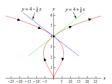
Note that there is apparently the potential for more than one tangent line here! We will look into this more after we’re done with the example.
The first thing that we should do is find the derivative so we can get the slope of the tangent line.
\[\frac{{dy}}{{dx}} = \frac{{\displaystyle \,\,\frac{{dy}}{{dt}}\,\,}}{{\displaystyle \,\,\frac{{dx}}{{dt}}\,\,}} = \frac{{2t}}{{5{t^4} - 12{t^2}}} = \frac{2}{{5{t^3} - 12t}}\]At this point we’ve got a small problem. The derivative is in terms of \(t\) and all we’ve got is an x-y coordinate pair. The next step then is to determine the value(s) of \(t\) which will give this point. We find these by plugging the \(x\) and \(y\) values into the parametric equations and solving for \(t\).
\[\begin{align*}0 & = {t^5} - 4{t^3} = {t^3}\left( {{t^2} - 4} \right) &\Rightarrow \hspace{0.25in} & t = 0, \pm 2\\ 4 & = {t^2} & \Rightarrow \hspace{0.25in} & t = \pm 2\end{align*}\]Any value of \(t\) which appears in both lists will give the point. So, since there are two values of \(t\) that give the point we will in fact get two tangent lines. That’s definitely not something that happened back in Calculus I and we’re going to need to look into this a little more. However, before we do that let’s actually get the tangent lines.
\(t = - 2:\)
Since we already know the \(x\) and \(y\)-coordinates of the point all that we need to do is find the slope of the tangent line.
The tangent line (at \(t = - 2\)) is then,
\[y = 4 - \frac{1}{8}x\]\(t = 2:\)
Again, all we need is the slope.
The tangent line (at \(t = 2\)) is then,
\[y = 4 + \frac{1}{8}x\]Before we leave this example let’s take a look at just how we could possibly get two tangents lines at a point. This was definitely not possible back in Calculus I where we first ran across tangent lines.
A quick graph of the parametric curve will explain what is going on here.

So, the parametric curve crosses itself! That explains how there can be more than one tangent line. There is one tangent line for each instance that the curve goes through the point.
The next topic that we need to discuss in this section is that of horizontal and vertical tangents. We can easily identify where these will occur (or at least the \(t\)’s that will give them) by looking at the derivative formula.
\[\frac{{dy}}{{dx}} = \frac{{\displaystyle \,\,\frac{{dy}}{{dt}}\,\,}}{{\displaystyle \,\,\frac{{dx}}{{dt}}\,\,}}\]Horizontal tangents will occur where the derivative is zero and that means that we’ll get horizontal tangent at values of \(t\) for which we have,
Horizontal Tangent for Parametric Equations
Vertical tangents will occur where the derivative is not defined and so we’ll get vertical tangents at values of \(t\) for which we have,
Vertical Tangent for Parametric Equations
Let’s take a quick look at an example of this.
We’ll first need the derivatives of the parametric equations.
\[\frac{{dx}}{{dt}} = 3{t^2} - 3 = 3\left( {{t^2} - 1} \right)\hspace{0.5in}\frac{{dy}}{{dt}} = 6t\]Horizontal Tangents
We’ll have horizontal tangents where,
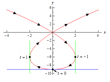
Now, this is the value of \(t\) which gives the horizontal tangents and we were asked to find the x-y coordinates of the point. To get these we just need to plug \(t\) into the parametric equations. Therefore, the only horizontal tangent will occur at the point \(\left( {0, - 9} \right)\).
Vertical Tangents
In this case we need to solve,
The two vertical tangents will occur at the points \(\left( {2, - 6} \right)\) and \(\left( { - 2, - 6} \right)\).
For the sake of completeness and at least partial verification here is the sketch of the parametric curve.

The final topic that we need to discuss in this section really isn’t related to tangent lines but does fit in nicely with the derivation of the derivative that we needed to get the slope of the tangent line.
Before moving into the new topic let’s first remind ourselves of the formula for the first derivative and in the process rewrite it slightly.
\[\frac{{dy}}{{dx}} = \frac{d}{{dx}}\left( y \right) = \frac{{\displaystyle \frac{d}{{dt}}\left( y \right)}}{{\displaystyle \frac{{dx}}{{dt}}}}\]Written in this way we can see that the formula actually tells us how to differentiate a function \(y\) (as a function of \(t\)) with respect to \(x\) (when \(x\) is also a function of \(t\)) when we are using parametric equations.
Now let’s move onto the final topic of this section. We would also like to know how to get the second derivative of \(y\) with respect to \(x\).
\[\frac{{{d^2}y}}{{d{x^2}}}\]Getting a formula for this is fairly simple if we remember the rewritten formula for the first derivative above.
Second Derivative for Parametric Equations
It is important to note that,
\[\frac{{{d^2}y}}{{d{x^2}}} \ne \frac{{\displaystyle \,\,\frac{{{d^2}y}}{{d{t^2}}}\,\,}}{{\displaystyle \,\,\frac{{{d^2}x}}{{d{t^2}}}\,\,}}\]Let’s work a quick example.
This is the set of parametric equations that we used in the first example and so we already have the following computations completed.
\[\frac{{dy}}{{dt}} = 2t\hspace{0.5in}\hspace{0.25in}\frac{{dx}}{{dt}} = 5{t^4} - 12{t^2}\hspace{0.5in}\frac{{dy}}{{dx}} = \frac{2}{{5{t^3} - 12t}}\]We will first need the following,
\[\frac{d}{{dt}}\left( {\frac{2}{{5{t^3} - 12t}}} \right) = \frac{{ - 2\left( {15{t^2} - 12} \right)}}{{{{\left( {5{t^3} - 12t} \right)}^2}}} = \frac{{24 - 30{t^2}}}{{{{\left( {5{t^3} - 12t} \right)}^2}}}\]The second derivative is then,
\[\begin{align*}\frac{{{d^2}y}}{{d{x^2}}} & = \frac{{\frac{d}{{dt}}\left( {\frac{{dy}}{{dx}}} \right)}}{{\frac{{dx}}{{dt}}}}\\ & = \frac{{\frac{{24 - 30{t^2}}}{{{{\left( {5{t^3} - 12t} \right)}^2}}}}}{{5{t^4} - 12{t^2}}}\\ & = \frac{{24 - 30{t^2}}}{{\left( {5{t^4} - 12{t^2}} \right){{\left( {5{t^3} - 12t} \right)}^2}}}\\ & = \frac{{24 - 30{t^2}}}{{t{{\left( {5{t^3} - 12t} \right)}^3}}}\end{align*}\]So, why would we want the second derivative? Well, recall from your Calculus I class that with the second derivative we can determine where a curve is concave up and concave down. We could do the same thing with parametric equations if we wanted to.
To compute the second derivative we’ll first need the following.
\[\frac{{dy}}{{dt}} = 7{t^6} + 5{t^4}\hspace{0.5in}\frac{{dx}}{{dt}} = - 2t\hspace{0.5in}\frac{{dy}}{{dx}} = \frac{{7{t^6} + 5{t^4}}}{{ - 2t}} = - \frac{1}{2}\left( {7{t^5} + 5{t^3}} \right)\]Note that we can also use the first derivative above to get some information about the increasing/decreasing nature of the curve as well. In this case it looks like the parametric curve will be increasing if \(t < 0\) and decreasing if \(t > 0\).
Now let’s move on to the second derivative.
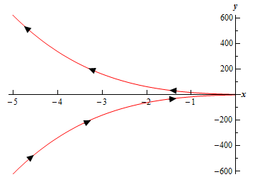
\[\frac{{{d^2}y}}{{d{x^2}}} = \frac{{ - \frac{1}{2}\left( {35{t^4} + 15{t^2}} \right)}}{{ - 2t}} = \frac{1}{4}\left( {35{t^3} + 15t} \right)\]It’s clear, hopefully, that the second derivative will only be zero at \(t = 0\). Using this we can see that the second derivative will be negative if \(t < 0\) and positive if \(t > 0\). So the parametric curve will be concave down for \(t < 0\) and concave up for \(t > 0\).
Here is a sketch of the curve for completeness sake.
