Section 9.1 : Parametric Equations and Curves
3. Eliminate the parameter for the following set of parametric equations, sketch the graph of the parametric curve and give any limits that might exist on \(x\) and \(y\).
\[x = \sqrt {t + 1} \hspace{0.5in}y = \frac{1}{{t + 1}}\hspace{0.5in}\hspace{0.5in}\,\,\,t > - 1\]Show All Steps Hide All Steps
Start SolutionFirst, we’ll eliminate the parameter from this set of parametric equations. For this particular set of parametric equations that is actually really easy to do if we notice the following.
\[x = \sqrt {t + 1} \,\,\hspace{0.25in}\hspace{0.25in} \Rightarrow \hspace{0.25in}\hspace{0.25in}{x^2} = t + 1\]With this we can quickly convert the \(y\) equation to,
\[y = \frac{1}{{{x^2}}}\] Show Step 2At this point we can get limits on \(x\) and \(y\) pretty quickly so let’s do that.
First, we know that square roots always return positive values (or zero of course) and so from the \(x\) equation we see that we must have \(x > 0\). Note as well that this must be a strict inequality because the inequality restricting the range of \(t\)’s is also a strict inequality. In other words, because we aren’t allowing \(t = - 1\) we will never get \(x = 0\).
Speaking of which, you do see why we’ve restricted the \(t\)’s don’t you?
Now, from our restriction on \(t\) we know that \(t + 1 > 0\) and so from the \(y\) parametric equation we can see that we also must have \(y > 0\). This matches what we see from the equation without the parameter we found in Step 1.
So, putting all this together here are the limits on \(x\) and \(y\).
\[x > 0\hspace{0.25in}\hspace{0.25in}y > 0\]Note that for this problem these limits are important (or at least the \(x\) limits are important). Because of the \(x\) limit we get from the parametric equation we can see that we won’t have the full graph of the equation we found in the first step. All we will have is the portion that corresponds to \(x > 0\).
Show Step 3Before we sketch the graph of the parametric curve recall that all parametric curves have a direction of motion, i.e. the direction indicating increasing values of the parameter, \(t\) in this case.
There are several ways to get the direction of motion for the curve. One is to plug in values of \(t\) into the parametric equations to get some points that we can use to identify the direction of motion.
Here is a table of values for this set of parametric equations.
| \(t\) | \(x\) | \(y\) |
|---|---|---|
| -0.95 | 0.2236 | 20 |
| -0.75 | 0.5 | 4 |
| 0 | 1 | 1 |
| 2 | \(\sqrt 3 \) | \(\frac{1}{3}\) |
Note that there is an easier way (probably – it will depend on you of course) to determine direction of motion. Take a quick look at the \(x\) equation.
\[x = \sqrt {t + 1} \,\]Increasing the value of \(t\) will also cause \(t\) + 1 to increase and the square root will also increase (we can verify with a quick derivative/Calculus I analysis if we want to). This means that the graph must be tracing out from left to right as the table of values above in the table supports.
Likewise, we could use the \(y\) equation.
\[y = \frac{1}{{t + 1}}\]Again, we know that as \(t\) increases so does \(t\) + 1. Because the \(t\) + 1 is in the denominator we can further see that increasing this will cause the fraction, and hence \(y\), to decrease. This means that the graph must be tracing out from top to bottom as both the \(x\) equation and table of values supports.
Using a quick Calculus analysis of one, or both, of the parametric equations is often a better and easier method for determining the direction of motion for a parametric curve. For “simple” parametric equations we can often get the direction based on a quick glance at the parametric equations and it avoids having to pick “nice” values of \(t\) for a table.
Show Step 4Finally, here is a sketch of the parametric curve for this set of parametric equations.
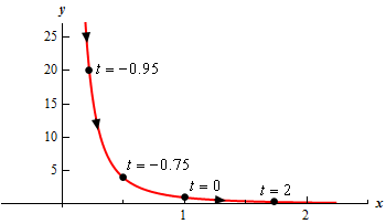
For this sketch we included the points from our table because we had them but we won’t always include them as we are often only interested in the sketch itself and the direction of motion.